38 excel bar graph labels

Excel 2019 - hw does one left-justify the text in an Excel horizontal ... • Excel 2019 (part of Office Professional Plus 2019) How graphic was created • Highlight desired data in Excel spreadsheet • From Excel ribbon - Insert chart - Bar - 100% Stacked Bar. One would think that by highlighting the label area text box and clicking on the alignment options, one could left-justify the text … nothing seems to work. How do I make excel label every bar in a bar chart? - Super User Insert->Pivot Chart; Click Clustered Column; Right-click on graph, select Format Axis; set specify unit interval to 1; Excel now just labels every 2nd bar, even though it would easily fit (I have about 150 bars) with the given label font size. Even though I have selected 1, it has the same text density as if I set specify unit interval to 2.

How to Make a Bar Chart in Microsoft Excel - How-To Geek Adding and Editing Axis Labels To add axis labels to your bar chart, select your chart and click the green "Chart Elements" icon (the "+" icon). From the "Chart Elements" menu, enable the "Axis Titles" checkbox. Axis labels should appear for both the x axis (at the bottom) and the y axis (on the left). These will appear as text boxes.

Excel bar graph labels

Create a Bar Chart in Excel (In Easy Steps) - Excel Easy Use a bar chart if you have large text labels. To create a bar chart, execute the following steps. 1. Select the range A1:B6. 2. On the Insert tab, in the Charts group, click the Column symbol. 3. Click Clustered Bar. 5/18 Completed! How to Make a Bar Graph in Excel: 9 Steps (with Pictures) - wikiHow Step 1, Open Microsoft Excel. It resembles a white "X" on a green background. A blank spreadsheet should open automatically, but you can go to File > New > Blank if you need to. If you want to create a graph from pre-existing data, instead double-click the Excel document that contains the data to open it and proceed to the next section.Step 2, Add labels for the graph's X- and Y-axes. To do so, click the A1 cell (X-axis) and type in a label, then do the same for the B1 cell (Y-axis). For ... how to add data labels into Excel graphs - storytelling with data There are a few different techniques we could use to create labels that look like this. Option 1: The "brute force" technique. The data labels for the two lines are not, technically, "data labels" at all. A text box was added to this graph, and then the numbers and category labels were simply typed in manually.

Excel bar graph labels. How to Make a Bar Chart in Excel | Smartsheet Right-click the axis, click Format Axis, click Text Box, and enter an angle. You can also opt to only show some of the axis labels. Right-click the axis, click Format Axis, then click Scale, and enter a value in the Interval between labels box. A value of 2 will show every other label; 3 will show every third. Histogram with Actual Bin Labels Between Bars - Peltier Tech Select the chart, then use Home tab > Paste dropdown > Paste Special to add the copied data as a new series, with category labels in the first column. You don't see the new series, because it's a series of bars with zero height. But you should notice that the wide bars have been squeezed a bit to make room for the added series. Bar Graph in Excel — All 4 Types Explained Easily - Simon Sez IT To create a simple bar graph, follow these steps: Get your Data ready. Make sure it has one categorical variable and one quantitative secondary variable. In my example from Sheet1, I have the time duration of 6 tasks. Select your Data with headers. Locate and click on the 2-D Clustered Bars option under the Charts group in the Insert Tab. Text Labels on a Horizontal Bar Chart in Excel - Peltier Tech On the Excel 2007 Chart Tools > Layout tab, click Axes, then Secondary Horizontal Axis, then Show Left to Right Axis. Now the chart has four axes. We want the Rating labels at the bottom of the chart, and we'll place the numerical axis at the top before we hide it. In turn, select the left and right vertical axes.

How to Add Axis Labels in Excel Charts - Step-by-Step (2022) - Spreadsheeto How to add axis titles 1. Left-click the Excel chart. 2. Click the plus button in the upper right corner of the chart. 3. Click Axis Titles to put a checkmark in the axis title checkbox. This will display axis titles. 4. Click the added axis title text box to write your axis label. How to Use Cell Values for Excel Chart Labels - How-To Geek Select the chart, choose the "Chart Elements" option, click the "Data Labels" arrow, and then "More Options." Uncheck the "Value" box and check the "Value From Cells" box. Select cells C2:C6 to use for the data label range and then click the "OK" button. The values from these cells are now used for the chart data labels. HOW TO CREATE A BAR CHART WITH LABELS INSIDE BARS IN EXCEL - simplexCT In the chart, right-click the Series "# Footballers" Data Labels and then, on the short-cut menu, click Format Data Labels. 8. In the Format Data Labels pane, under Label Options selected, set the Label Position to Inside End . Edit titles or data labels in a chart - support.microsoft.com The first click selects the data labels for the whole data series, and the second click selects the individual data label. Right-click the data label, and then click Format Data Label or Format Data Labels. Click Label Options if it's not selected, and then select the Reset Label Text check box. Top of Page

How to Change Excel Chart Data Labels to Custom Values? - Chandoo.org First add data labels to the chart (Layout Ribbon > Data Labels) Define the new data label values in a bunch of cells, like this: Now, click on any data label. This will select "all" data labels. Now click once again. At this point excel will select only one data label. Go to Formula bar, press = and point to the cell where the data label ... How to label graphs in Excel | Think Outside The Slide If the values are needed, then you will want to use data labels. I suggest placing them inside the end of the column or bar, or just outside the column or bar. This example shows a column graph with data labels only. Example 1 If the message is more related to the ranking of the values, then you can use an axis. Create a multi-level category chart in Excel - ExtendOffice Select the dots, click the Chart Elements button, and then check the Data Labels box. 23. Right click the data labels and select Format Data Labels from the right-clicking menu. 24. In the Format Data Labels pane, please do as follows. 24.1) Check the Value From Cells box; Bar Chart in Excel (Examples) | How to Create Bar Chart in Excel? - EDUCBA Bar Chart in Excel is one of the easiest types of the chart to prepare by just selecting the parameters and values available against them. We must have at least one value for each parameter. Bar Chart is shown horizontally, keeping their base of the bars at Y-Axis.

34 How To Label Bar Graph In Excel - Labels Design Ideas 2020

Excel charts: add title, customize chart axis, legend and data labels Click anywhere within your Excel chart, then click the Chart Elements button and check the Axis Titles box. If you want to display the title only for one axis, either horizontal or vertical, click the arrow next to Axis Titles and clear one of the boxes: Click the axis title box on the chart, and type the text.

Quickly create a bar graph with interval labels in Excel

Bar Chart in Excel | Examples to Create 3 Types of Bar Charts We will add "Data Labels" to the data series in the plotted area. We will click on the chart area to select the data series. Now, as shown in the screenshot, we will right-click on the data series and choose the add data labels to add the data label option. We can move the bar chart to the desired place in the worksheet.

How to Create a Bar Chart With Labels Above Bars in Excel

Every-other vertical axis label for my bar graph is being skipped 2. Make sure that interval between the labels is set to 1 point in the vertical axis. The Format Axis dialog box appears. From the Categories list, select Scale > The Format Axis dialog box refreshes to display the Scale options > To change the minimum value of the y-axis, in the Minimum text box, type the minimum value (1.0) you want the y ...

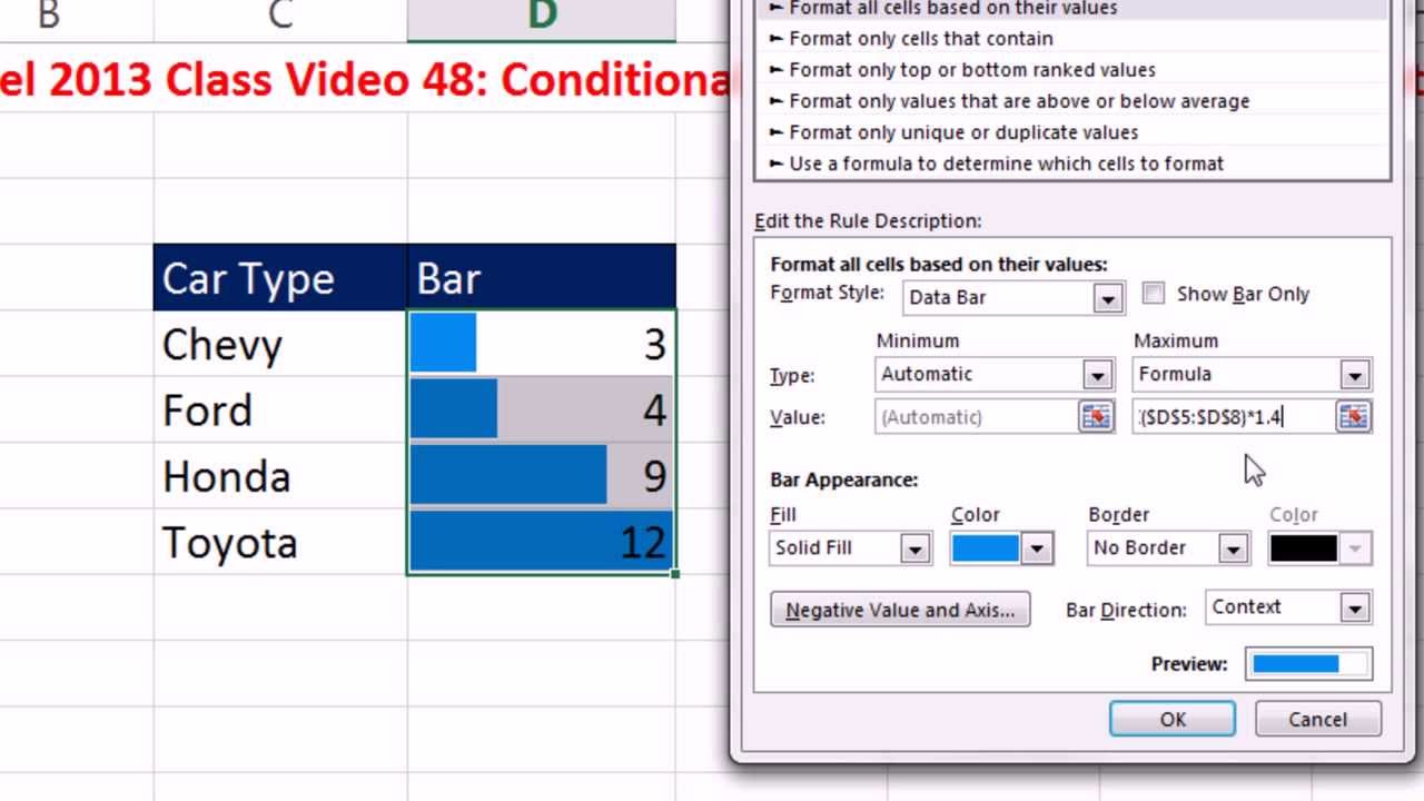
Highline Excel 2013 Class Video 48: Conditional Formatting: Bar Chart with Data Labels - YouTube

HOW TO CREATE A BAR CHART WITH LABELS ABOVE BAR IN EXCEL - simplexCT HOW TO CREATE A BAR CHART WITH LABELS ABOVE BAR IN EXCEL 1. Highlight the range A5:B16 and then, on the Insert tab, in the Charts group, click Insert Column or Bar Chart >... 2. Next, lets do some cleaning. Delete the vertical gridlines, the horizontal value axis and the vertical category axis. 3. ...

How to label graphs in Excel | Think Outside The Slide

Add or remove data labels in a chart - support.microsoft.com To label one data point, after clicking the series, click that data point. In the upper right corner, next to the chart, click Add Chart Element > Data Labels. To change the location, click the arrow, and choose an option. If you want to show your data label inside a text bubble shape, click Data Callout.

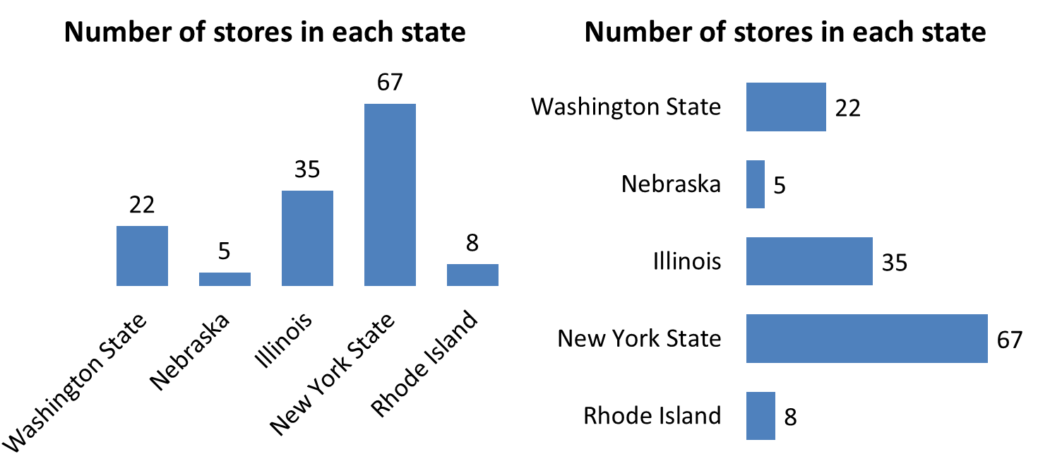
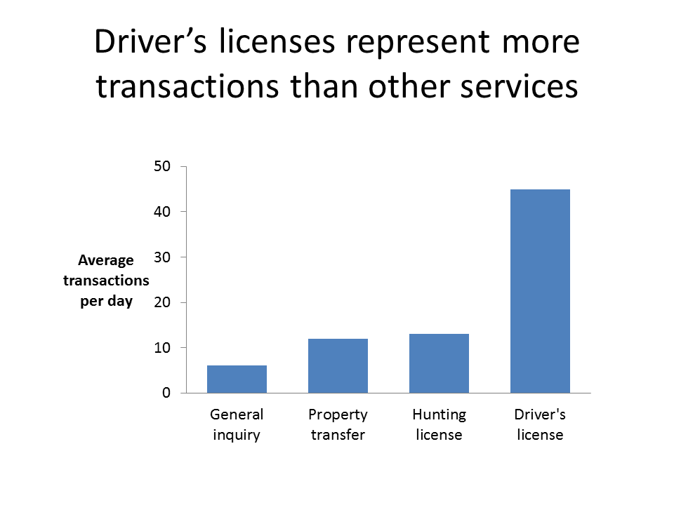
Column Graphs vs. Bar Charts – When to choose each one | Think Outside The Slide

How to group (two-level) axis labels in a chart in Excel? - ExtendOffice The Pivot Chart tool is so powerful that it can help you to create a chart with one kind of labels grouped by another kind of labels in a two-lever axis easily in Excel. You can do as follows: 1. Create a Pivot Chart with selecting the source data, and: (1) In Excel 2007 and 2010, clicking the PivotTable > PivotChart in the Tables group on the Insert Tab;

Add Total Label On Stacked Bar Chart In Excel - YouTube

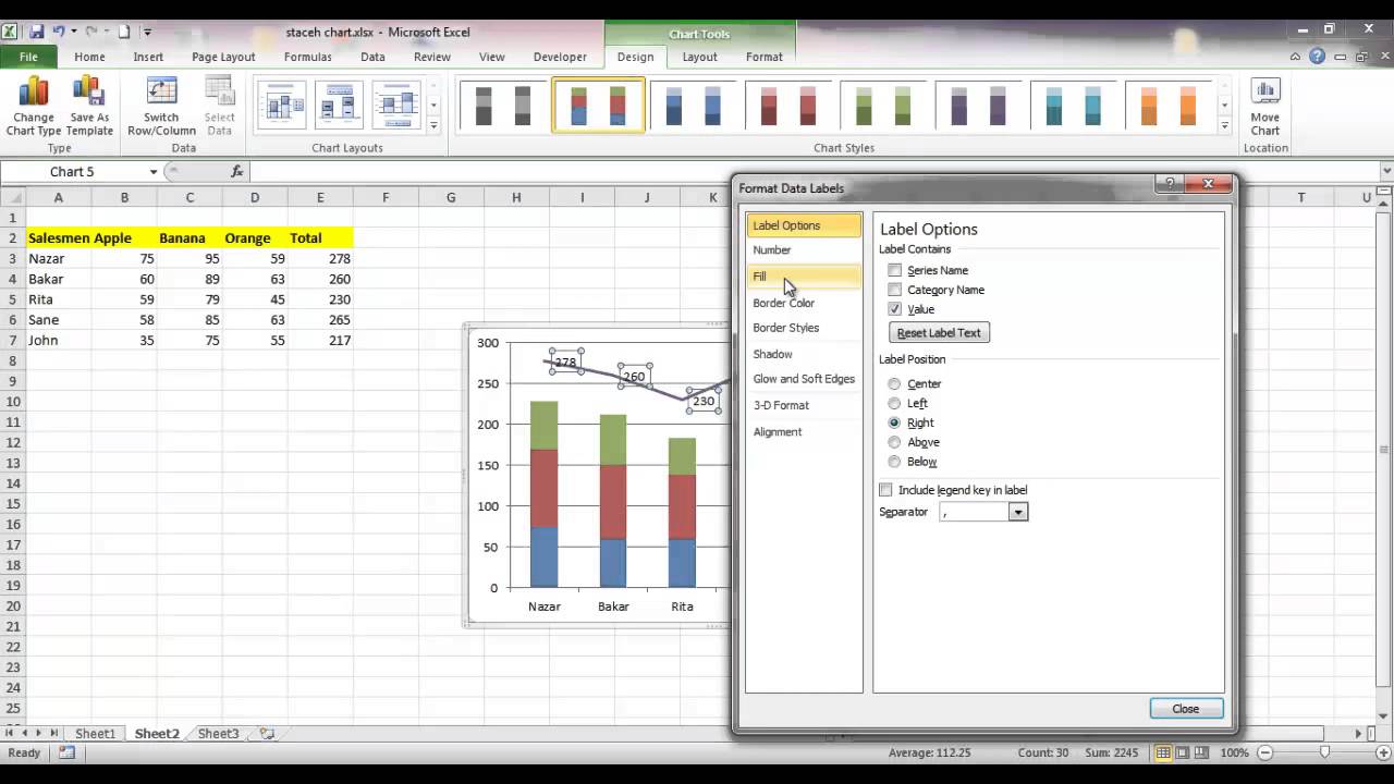
How to Add Total Data Labels to the Excel Stacked Bar Chart For stacked bar charts, Excel 2010 allows you to add data labels only to the individual components of the stacked bar chart. The basic chart function does not allow you to add a total data label that accounts for the sum of the individual components. Fortunately, creating these labels manually is a fairly simply process.

How to label graphs in Excel | Think Outside The Slide

Bugs with Excel bar chart data labels - Microsoft Community In reply to Prof Dominic Foo's post on March 10, 2016. You could use some code to reset them. Something like this (untested): Option Explicit. Type dlFormatting. AutoText As Boolean. NumberFormat As String. Position As XlDataLabelPosition. Separator As String.

Text Labels on a Horizontal Bar Chart in Excel - Peltier Tech Blog

How to Add Percentages to Excel Bar Chart - Excel Tutorials If we would like to add percentages to our bar chart, we would need to have percentages in the table in the first place. We will create a column right to the column points in which we would divide the points of each player with the total points of all players. We will select range A1:C8 and go to Insert >> Charts >> 2-D Column >> Stacked Column:

Formatting Charts

How to Add Total Values to Stacked Bar Chart in Excel Step 4: Add Total Values. Next, right click on the yellow line and click Add Data Labels. Next, double click on any of the labels. In the new panel that appears, check the button next to Above for the Label Position: Next, double click on the yellow line in the chart. In the new panel that appears, check the button next to No line:

EXCEL : BROKEN COLUMN AND BAR CHARTS

how to add data labels into Excel graphs - storytelling with data There are a few different techniques we could use to create labels that look like this. Option 1: The "brute force" technique. The data labels for the two lines are not, technically, "data labels" at all. A text box was added to this graph, and then the numbers and category labels were simply typed in manually.

How to label graphs in Excel | Think Outside The Slide

How to Make a Bar Graph in Excel: 9 Steps (with Pictures) - wikiHow Step 1, Open Microsoft Excel. It resembles a white "X" on a green background. A blank spreadsheet should open automatically, but you can go to File > New > Blank if you need to. If you want to create a graph from pre-existing data, instead double-click the Excel document that contains the data to open it and proceed to the next section.Step 2, Add labels for the graph's X- and Y-axes. To do so, click the A1 cell (X-axis) and type in a label, then do the same for the B1 cell (Y-axis). For ...